Two Old Draft Posts from My LIDAR Study

Note: I had two draft posts from my Lidar study last Summer that are incomplete, but contain useful information I will want to refer to in the future.  Since time does not allow me to complete them now, I'll just publish them both "as is" here...

Visualizing the Loudoun County Lidar Data

Data

For the PV Viability Map project, we are using Lidar data from Loudoun County, Virginia.  Loudoun County was chosen because the goal of the initiating organization, Northern Virginia Regional Commision (NVRC), is to produce a map for all the NVRC members, but complete Lidar data is currently only available for Loudoun County.  Currently available data can be obtained from the USGS EarthExplorer website (see previous post, Getting Started with LIDAR Data), but it is available in small distribution units from the VirginiaLidar site.  A few other websites I came across in searching that might be useful later include:

• The National Map [USGS]
• Center for LIDAR Information Coordination and Knowledge (CLICK) [USGS]

To get the data we'll be using, I went to this folder on Virginia Lidar's Google drive.  I downloaded the PDF, Shapefile zip, and KMZ files.  This is the first time I've encountered KMZ files, which are zipped Keyhole Markup Language files.  KML is an open standard for expressing annotations and markers on web based 2D and 3D maps.  It appears you can work with them in OpenStreetMap.

The Lidar data on the Virginia Lidar site is divided into blocks.  The region covered by each block is described in the LoudounCo_Ref.pdf PDF file in the Virginia Lidar Google drive location linked above.  Here is what it looks like:

To begin learning to work with the data, I set myself the task of downloading a single block of the data and then exploring tools to visualize it.  I choose 18STJ7733.laz since it contains the intersection of Routes 15 and 7 in downtown Leesburg (see this Google map), and would thus I hoped have recognizable features that would aid in testing the visualizations. Since the data is provided in compressed LAZ format, and many of the tools require the uncompressed LAS format, I had to first uncompress the file. I described how I did this in an earlier post.

Visualization

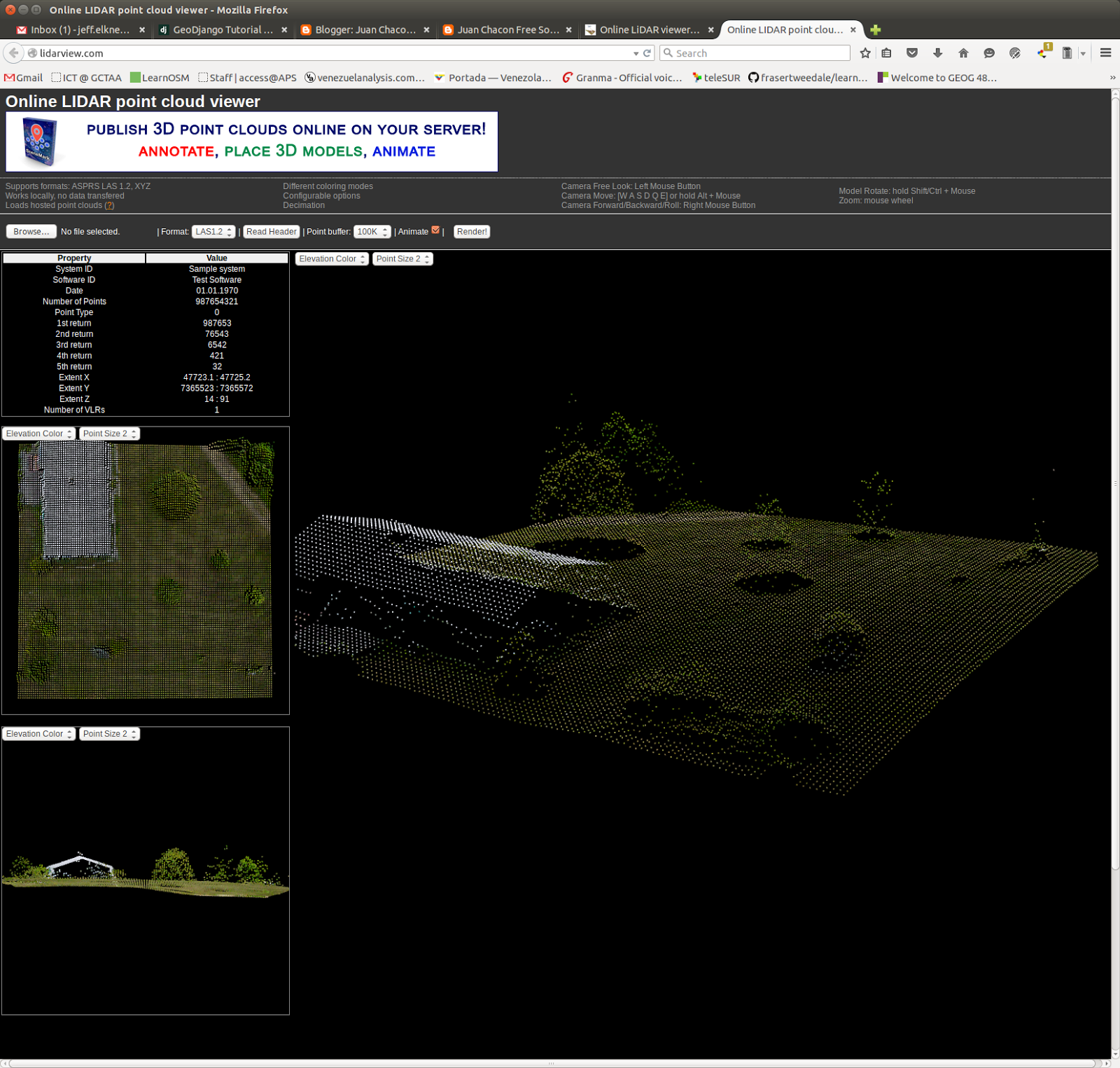
After spending a reasonable amount of time searching on the web for Lidar visualization tools, it became clear to me that I will have to overcome a number of obstacles to be able to work with this data.  I'm going to need to understand the LAS file format in some detail to use the lower level tools that are available for GNU/Linux systems.  I may explore some of the free software tools that are only available for Windows, but I'll only do that after I've exhausted what I can do a free software platform.

I found a website, http://lidarview.com, that offers through the web visualization of LAS files.  This screenshot shows the website with the default data being visualized:

 

Manual of Airborne Topographic Lidar - Chapter 3 Notes

Chapter 3 of the Manual of Airborne Topographic Lidar is titled Enabling Technologies, and discusses the Global Navigation Satellite Systems (GNSS) and inertial navigation systems (INS) that together enable airborne laser scanning (ALS).  Both these technologies were mentioned frequently in the chapter 2 discussion of elements of ALS technologies, and it is clear from the discussion why ALS could not emerge as a viable commercial technology until the 1990s, when the GPS system become available.

Global Navigation Satellite Systems

There are currently two operational GNSS systems, the US Global Positioning System (GPS), and the Russian GLObal NAvigation Satellite System (GLONASS), and two systems under development, the EU Galileo system, and the Chinese BeiDou Navigation Satellite System (BDS), both expected to be completed by 2020.

How Does a GNSS Work? 

The text describes GNSS as "a constellation of satellites carrying atomic clocks that broadcast time and an arbitrary number of receivers each of which computes its own position on the Earth from measured signal propagation times from the visible satellites to the receiver." (p. 99).  What I didn't understand was how the receiver could compute the propagation time of the signal (and thus find the distance from the satellite) without having a clock that was synchronized with the atomic clock on the satellite.  A space.stackexchange.com post titled How does GPS receiver synchronize time with GPS satellites? provides a nice explaination:

"The time value isn't used to tell the receiver what time it is (at least not directly, although that is helpful later). It's used so that the receiver can tell relatively what the distance is to each satellite.

If you hear Sat A say that the time is 0.00000 and Sat B says the time is 0.00010, then if they are in sync, you must be closer to B than to A. You can tell exactly how much closer you are by the specific time difference.

Repeat the calculations with a few other satellites and you will find that there is only one place (and time) that the receiver can be located.

The GPS receiver computes a solution that simultaneously provides Position, Velocity, and Time (PVT). It's not that one is calculated first, then the other is. They all fall out simultaneously."

A bit later in the post the following equation is listed:


Looking at the 4 unknowns, x, y, z, and t, it makes sense why 4 satellites are need to provide a location (and time).

Resources

• How does GPS work? (physics.org)